digital signal processing - notes 2

digital signal processing - notes 2 - vector spaces

discrete signal vectors
- vector space framework
vector spaces
signal spaces
- completeness
- common signal spaces
bases
subspaces
references

discrete signal vectors

a generic discrete signal:
- \( x[n] = …,1.23, -0.73, 0.89, 0.17, -1.15, -0.26,… \)
- set of ordered number sequence
four classes of signals
- finite length
- infinite length
- periodic
- finite support
digital signal processing:
- signal analysis
- signal synthesis
number sets:
- \( \mathbb{N} \): natural numbers \( [1,\infty) \)
  - whole numbers \( [0,\infty) \)
- \( \mathbb{Z} \): integers
- \( \mathbb{Q} \): rational numbers
  - inclusive of recurring mantissa
- \( \mathbb{P} \): irrational numbers
  - non-repeating and non-recurring mantissa
  - \( \pi \) value, \( \sqrt{2} \)
- \( \mathbb{R} \): real numbers (everything on the number line)
  - includes rational and irrational numbers
- \( \mathbb{C} \): complex numbers
  - includes real and imaginary numbers

number-sets

fig: number sets

vector space framework:

justification for dsp application:
- common framework for various signal classes
  - inclusive of continuous-time signals
- easy explanation of Fourier Transform
- easy explanation of sampling and interpolation
- useful in approximation and compression
- fundamental to communication system design
paradigms for vector space application to discrete signals
- object oriented programming
  - the instantiated object can have unique property values
  - but for a given object class, the properties and methods are the same
- lego
  - various unit blocks, same and different
  - units assembled in different ways to build different complex structures
  - similarly, a complex signal is broken down into a combination of basis vectors for analysis
key takeaways
- vector spaces are general objects
- vector spaces are defined by their properties
- once signal properties satisfy vector space conditions
  - vector space tools can be applied to signals

vector spaces

some vector spaces
- \(\mathbb{R}^2\): 2D space
- \(\mathbb{R}^3\): 3D space
- \(\mathbb{R}^N\): N real numbers
- \(\mathbb{C}^N\): N complex numbers
- \(\ell_2(\mathbb{Z}) \):
  - square-summable infinite sequences
- \(L_2([a,b]) \):
  - square-integrable functions over interval \([a,b] \)
vector spaces can be diverse
some vector spaces can be represented graphically
- helps visualize the signal for analysis insights
\(\mathbb{R}^2\): \(\textbf{x} = [x_0, x_1]^T\)
\(\mathbb{R}^3\): \(\textbf{x} = [x_0, x_1, x_2]^T\)
- both can be visualized in a cartesian system
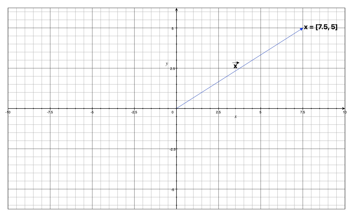
fig: vector in 2D space
\(L_2([a,b]) \): \( \textbf{x} = x(t), t \in [-1,1] \)
- function vector space
- can be represented as sine wave along time
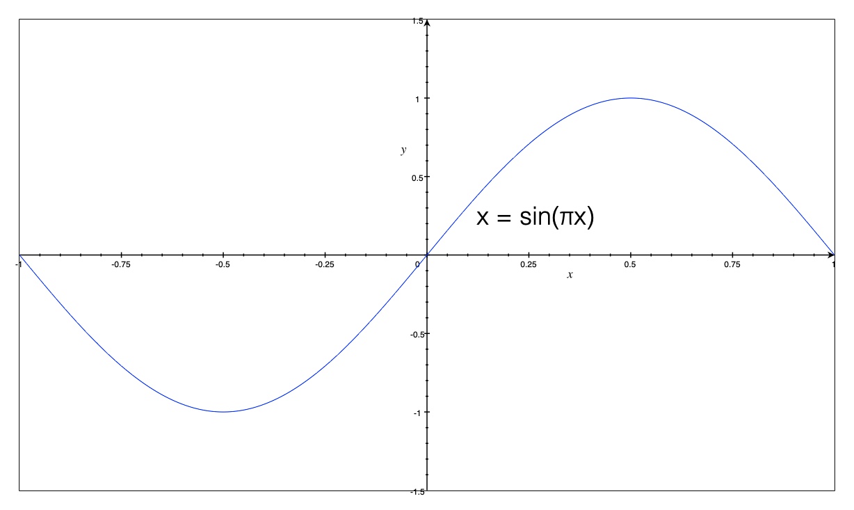
fig: L2 function vector
others cannot be represented graphically:
- \(\mathbb{R}^N\) for \( N > 3\)
- \(\mathbb{C}^N\) for \( N > 1\)

vector space axioms

informally, a vector space:
- has vectors in it
- has scalars in it, like \( \mathbb{C} \)
- scalers must be able to scale vectors
- vector summation must work
formally, \( \forall \text{ } \textbf{x,y,z} \in V, \text{ } and \text{ } \alpha, \beta \in \mathbb{C} \) (\(V\): vector space)
- \(\textbf{x} + \textbf{y} = \textbf{y} + \textbf{x}\)
  - commutative addition
- \( (\textbf{x} + \textbf{y}) + \textbf{z} = \textbf{x} + (\textbf{y} + \textbf{z})\)
  - distributive addition
- \( \alpha(\textbf{x} + \textbf{y}) = \alpha \textbf{y} + \alpha \textbf{x}\)
  - distributive scalar multiplication over vectors
- \( (\alpha + \beta)\textbf{x} = \alpha \textbf{x} + \beta \textbf{x} \)
  - distributive vector multiplication over scalers
- \( \alpha(\beta \textbf{x}) = \alpha(\beta \textbf{x})\)
  - associative scalar multiplication
- \( \exists \text{ } 0 \in V \text{ } | \text{ } \textbf{x} + 0 = 0 + \textbf{x} = \textbf{x} \)
  - null vector, \( 0 \), exists
  - addition of \( 0 \) and another vector \(\textbf{x}\) returns \(\textbf{x}\)
  - summation with null vector is commutative
- \( \forall \text{ } \textbf{x} \in V \text{ } \exists \text{ } (-\textbf{x}) \text{ } | \text{ } \textbf{x} + (-x) = 0 \)
  - an inverse vector exists in vector space such that adding the vector with it’s inverse yields the null vector
examples:
- \( \mathbb{R}^N \): vector of N real numbers
  - two vectors from this space look like:
    - \(\textbf{x} = [x_0, x_1, x_2, … x_N]^T \)
    - \(\textbf{y} = [x_0, x_1, x_2, … x_N]^T \)
  - the above mentioned rules apply to these vectors and can be verified
- \( L_2[-1,1] \)

inner product

aka dot product: measure of similarity of two vectors
- \( \langle \cdot, \cdot \rangle: V \times V \rightarrow \mathbb{C} \)
takes two vectors and outputs a scaler which indicates how similar the two vectors are
inner product axioms
- \( \langle x+y, z \rangle = \langle x, z \rangle + \langle y, z \rangle\)
  - distributive over vector addition
- \( \langle x,y \rangle = \langle y,x \rangle^* \)
  - commutative with conjugation
- \( \langle x, \alpha y \rangle = \alpha \langle x,y \rangle \)
  - distributive with scalar multiplication
  - when scalar scales the second operand
- \( \langle \alpha x,y \rangle = \alpha^* \langle x,y \rangle \)
  - distributive with scalar multiplication
  - conjugate scalar if it scaling the first operand
- \( \langle x,x \rangle \geq 0 \)
  - self inner product \( \in \mathbb{R}\)
- \( \langle x,x \rangle = 0 \Leftrightarrow x = 0 \)
  - if self inner product is 0, then the vector is the null vector
- if \( \langle x,y \rangle = 0 \text{ } and \text{ } x,y \neq 0 \),
  - then \( x \) and \( y \) are orthogonal
inner product is computed differently for different vector spaces
in \( \mathbb{R}^2 \) vector space:
- \( \langle x,y \rangle = x_0y_0 + x_1y_1 = \Vert x \Vert \Vert y \Vert \cos \alpha\)
  - where \( \alpha\): angle between \(x\) and \(y\)
- when two vectors are orthogonal to each other
  - \( \alpha = 90^{\circ}\), so \( \cos 90^{\circ} = 0 \), so \( \langle x,y\rangle = 0\)
in \( L_2[-1,1]\) vector space:
- \( \langle x,y \rangle = \int_{-1}^1 x(t) y(t) dt\)
  - norm: \( \langle x,x \rangle = \Vert x \Vert^2 = \int_{-1}^1 \sin^2(\pi t)dt \)
- the inner product of a symmetric and an anti-symmetric function is 0
  - i.e. they are orthogonal to each other and cannot be expressed as a factor of the other in any way
  - example 1:
    - \( x = \sin(\pi t) \) - anti-symmetric
    - \( y = 1 - \vert t \vert\) - symmetric
    - \( \langle x,y \rangle = \int_{-1}^1 (\sin(\pi t))(1 - \vert t \vert) dt = 0 \)
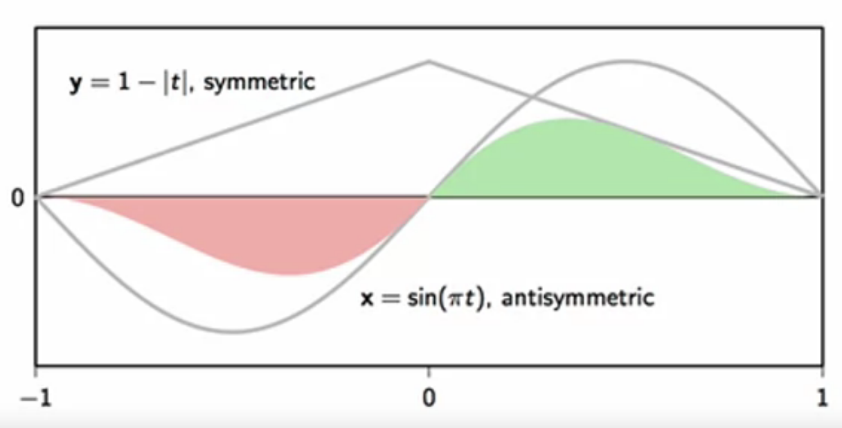
  fig: inner product of a symmetric and an anti-symmetric function
  - example 2:
    - \( x = \sin( 4 \pi t)\)
    - \( y = \sin( 5 \pi t)\)
    - \( \langle x,y \rangle = \int_{-1}^1 (\sin(4 \pi t))(\sin(5 \pi t)) dt = 0 \)

norm and distance

norm of a vector:
- inner product of a vector with itself
  - square of the norm (length) of a vector
- \( \langle x,x \rangle = x_0^2 + x_1^2 = \Vert x \Vert ^ 2 \)

distance between two vectors:
- the norm of the difference of the two vectors
the distance between orthogonal vectors is not zero

in \( \mathbb{R}^2 \), norm is the distance between the vector end points
- \( \Vert x - y \Vert \) is the difference vector
- \( \Vert x - y \Vert = \sqrt{(x_0 - y_0)^2 + (x_1 - y_1)^2} \)
  - connects the end points of the vectors \(x \) and \(y \)
- see triangle rule of vector addition, and pythagorean theorem
in \( L_2[-1,1] \), the norm is the mean-squared error:
- \( \int_{-1}^1 \vert x(t) - y(t) \vert^2 dt \)

signal spaces

completeness

consider an infinite sequence of vectors in a vector space
if it converges to a limit within the vector space
- then said vector space is “complete”
- also called Hilbert Space
limiting operation is ambiguous, definition varies from one space to the other
so some limiting operation may fail and point outside the vector space
- such vector spaces are not said to be complete

common signal spaces

while vectors spaces can be applied to signal processing
- not all vector spaces can be used for all signals
different signal classes are managed in different spaces

\( \mathbb{C}^N \): vector space of N complex tuples
- valid signal space for finite length signals
  - vector notation: \(\textbf{x} = [x_0, x_1, … x_N]^T\)
  - where \( x_0, x_1 … x_N \) are complex tuples
- also valid for periodic signals
  - vector notation: \( \tilde{\textbf{x}}\)
- all operations are well defined and intuitive
- inner product: \( \langle \textbf{x,y} \rangle = \sum_{n=0}^{N-1} x^*[n]y[n] \)
  - well defined for all finite-length vectors in \( \mathbb{C}^N\)
the inner product for infinite length signals explode in \( \mathbb{C}^N\)
- inappropriate for infinite length signal analysis

\( \ell_2(\mathbb{Z}) \): vector space of square-summable sequences
- requirement for sequences to be square-summable:
  - \( \sum \vert x[n] \vert^2 < \infty\)
  - sum of squares of elements of the sequence is less than infinity
  - all sequences that live in this space must have finite energy
- “well-behaved” infinite-length signals live in \( \ell_2(\mathbb{Z}) \)
  - vector notation: \(\textbf{x} = […, x_{-2}, x_{-1}, x_0, x_1, … ]^T\)

lot of other interesting infinite length signals do not live in \( \ell_2 \)
- examples:
  - \(x[n] = 1 \)
  - \(x[n] = \cos(\omega n) \)
- these have to be dealt with case-by-case

basis

a basis is a building block of a vector space
- a vector space usually has a few basis vectors called bases
- like the lego unit blocks
any element in a vector space can be
- built with a combination of these bases
- decomposed into a linear combination of these bases
the basis of a space is a family of vectors which are least like each other
- but they all belong to the same space
- as a linear combination, the basis vectors capture all the information within their vector space
fourier transform is simply a change of basis

vector families

\( \{ \textbf{w}^{(k)} \} \): family of vectors
- \( k \): index of the basis in the family

canonical \(\mathbb{R}^2\) basis: \( \textbf{e}^k\)
- \( \textbf{e}^{(0)} = \begin{bmatrix} 1\\ 0 \end{bmatrix} \text{; } \textbf{e}^{(1)} = \begin{bmatrix} 0\\ 1 \end{bmatrix} \)
- this family of basis vectors is denoted by \( \textbf{e}^k\)
any vector can be expressed as a linear combination of \( \textbf{e}^k\) in \( \mathbb{R}^2 \)
- \( \begin{bmatrix} x_0 \\ x_1 \end{bmatrix} = x_0\begin{bmatrix} 1 \\ 0 \end{bmatrix} + x_1\begin{bmatrix} 0 \\ 1 \end{bmatrix} \)
- \( \textbf{x} = x_0 \textbf{e}^{(0)} + x_1 \textbf{e}^{(1)}\)
graphical example:
- \( \begin{bmatrix} 2 \\ 1 \end{bmatrix} = 2\begin{bmatrix} 1 \\ 0 \end{bmatrix} + 1\begin{bmatrix} 0 \\ 1 \end{bmatrix} \)
- \( \textbf{x} = 2 \textbf{e}^{(0)} + 1 \textbf{e}^{(1)}\)

R2-basis

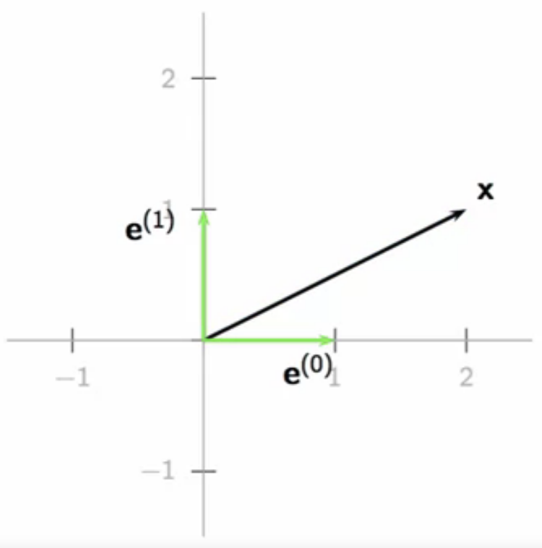
fig: linear combination of canonical \( \textbf{e}^k\) in \(\mathbb{R}^2\)

non-canonical \(\mathbb{R}^2\) basis example: \( \textbf{v}^k\)
- \( \textbf{v}^{(0)} = \begin{bmatrix} 1\\ 0 \end{bmatrix} \text{; } \textbf{v}^{(1)} = \begin{bmatrix} 1\\ 1 \end{bmatrix} \)
any vector can be expressed as a linear combination of these vectors in \(\mathbb{R}^2\)
- the coefficients of the bases will be different compared to the canonical bases
graphical example:
- \( \begin{bmatrix} 2 \\ 1 \end{bmatrix} = \alpha \textbf{v}^{(0)} + \beta \textbf{v}^{(1)} \)
- \( \begin{bmatrix} 2 \\ 1 \end{bmatrix} = \alpha \begin{bmatrix} 1\\ 0 \end{bmatrix} + \beta \begin{bmatrix} 1\\ 1 \end{bmatrix} \)
  - by rule of parallelogram vector addition
- \( \alpha = 1 \text{; } \beta = 1\)

R2-basis

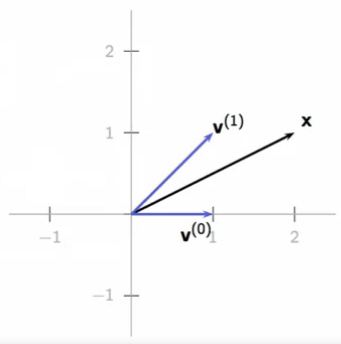
fig: linear combination of non-canonical \( \textbf{v}^k\) in \(\mathbb{R}^2\)

only vectors which are linearly independent can be the basis vectors of a space

infinite dimensional spaces bases:
- some limitations have to be applied to obtain basis vectors of infinite dimension
- \( \textbf{x} = \sum_{k=0}^{\infty} \alpha_k \textbf{w}^{(k)} \)
a canonical basis of \(\ell_2(\mathbb{Z})\)
- \( \textbf{e}^{k} = \begin{bmatrix} .\\.\\.\\ 0\\ 0\\ 1\\ 0\\ 0\\ 0\\ .\\.\\.\\ \end{bmatrix} \), \(k\) -th position, \( k \in \mathbb{Z} \)

function vector spaces:
- basis vector for functions: \( f(t) = \sum_{k}\alpha_{k}\textbf{h}^{(k)}(t) \)
the fourier basis for functions over an interval \([-1,1]\):
- \( \frac{1}{\sqrt{2}}, \cos\pi t, \sin\pi t, \cos2\pi t, \sin2\pi t,\cos3\pi t, \sin3\pi t, \ldots \)
- any square-integrable function in \([-1,1]\) can be represented as a linear combination of fourier bases
- a square wave can be expressed as a sum of sines

formally, in a vector space \( H \),
a set of \( K \) vectors from \(H\), \(W = \{ \textbf{w}^{(k)}\}_{k=0,1,\ldots,K-1} \) is a basis for \( H \) if:
1. \(\forall \in H \): \( \textbf{x} = \sum_{k=0}^{K-1}\alpha_k\textbf{w}^{(k)} \), \( \alpha_k \in \mathbb{C} \)
2. the coefficients \( \alpha_k\) are unique
  - this implies linear independence in the vector basis
  - \( \sum_{k=0}^{K-1} \alpha_k\textbf{w}^{(k)} = 0 \Leftrightarrow \alpha_k = 0, k=0,1,\ldots,K-1 \)

orthonormal basis

the orthogonal bases are the most important
- of all possible bases for a vector space
orthogonal basis: \( \langle \textbf{w}^{(k)},\textbf{w}^{(n)} \rangle = 0 \) for \( k \neq n\)
- vectors of an orthogonal basis are mutually orthogonal
- their inner product with each other is zero
in some spaces, the orthogonal bases are also orthonormal
- i.e. they are unit norm
- their length \( \Vert \textbf{w}^{(k)}\Vert = 1 \)
the inner product of any two vectors in the orthonormal bases is the difference between their indices
- \( \langle \textbf{w}^{(k)}, \textbf{w}^{(n)} \rangle = \delta[n-k]\)
gran-schmidt algorithm can be used to orthonormalize any orthogonal bases
obtaining the bases coefficients \( \alpha_k \) for bases can be involved and challenging
- \( \textbf{x} = \sum_{k=0}^{K-1} \alpha_k\textbf{w}^{(k)} \)
  - \( \textbf{x}\): a vector as the linear combination of \(K\) basis vectors \( \textbf{w}^{(k)} \),
  - with corresponding coefficients \( \alpha_k \)
- however, they are easy to obtain with an orthonormal basis
  - \( \alpha_k = \langle \textbf{w}^{(k)},\textbf{x} \rangle\)

change of basis

\( \textbf{x} = \sum_{k=0}^{K-1} \alpha_k\textbf{w}^{(k)} = \sum_{k=0}^{K-1} \beta_k\textbf{v}^{(k)}\)
- \( \textbf{v}^{(k )}\) is the target basis, \(\textbf{w}^{(k )}\) is the original basis
if \( \{ \textbf{v}^{(k )} \} \) is orthonormal:
- \( \beta_h = \langle v^{(h)}, \textbf{x} \rangle \)
- \( = \langle \textbf{v}^{(h)}, \sum_{k=0}^{K-1} \alpha_k\textbf{w}^{(k)} \rangle \)
- \( = \sum_{k=0}^{K-1} \alpha_k \langle \textbf{v}^{(h)}, \textbf{w}^{(k)} \rangle \)
- \( = \sum_{k=0}^{K-1} \alpha_k c_{hk} \)
- \( = \begin{bmatrix} c_{00} & c_{01} & \ldots & c_{0(K-1)}\\ & & \vdots & \\ c_{(K-1)0} & c_{(K-1)1} & \ldots & c_{(K-1)(K-1)} \end{bmatrix} \begin{bmatrix} \alpha_0\\ \vdots\\ \alpha_{K-1} \end{bmatrix}\)
this forms the core of the discrete fourier transform algorithm for finite length signals
can be applied to elementary rotations of basis vectors in the euclidean plane
- the same vector has different coefficients in the original and the rotates bases
- the rotation matrix is obtained by the matrix multiplication of the original and the target bases
- the rotation matrix applied to a vector in the original bases yields the coefficients of the same vector in the rotated bases
- the matrix multiplication of the rotation matrix with its inverse yields the identity matrix

subspaces

subspaces can be applied to signal approximation and compression
with vector \( \textbf{x} \in V \) and subspace \(S \subseteq V \)
- approximate \( \textbf{x} \) with \( \hat{\textbf{x}} \in S \) by
- take projection of the vector \(\textbf{x}\) in \( V \) on \( S \)
due to the adaptation of vector space paradigm for signal processing
- this geometric intuition for approximation can be extended to arbitrarily complex vector spaces

vector subspace

a subspace is a subset of vectors of a vector space closed under addition and scalar multiplication
classic example:
- \( \mathbb{R}^2 \subset \mathbb{R}^3 \)
- in-plane vector addition and scalar multiplication operations do not result in vectors outside the plane
- \( \mathbb{R}^2 \) uses only 2 of the 3 orthonormal basis of \( \mathbb{R}^3\)
the subspace concept can be extended to other vector spaces
- \(L_2[-1,1]\): function vector space
  - subspace: set of symmetric functions in \(L_2[-1,1]\)
  - when two symmetric functions are added, they yield symmetric functions
subspaces have their own bases
- a subset of their parent space’s bases

least square approximations

\( \{ \textbf{s}^{(k)} \}_{k=0,1,\ldots,K-1} \) orthonormal basis for \( S \)
orthogonal projection:
- \( \hat{\textbf{x}} = \sum_{k=0}^{K-1} \langle \textbf{s}^{(k)},\textbf{x} \rangle \textbf{s}^{(k)} \)
the orthogonal projection: the “best” approximation of \( \textbf{x} \) over \(S\)
- because of two of its properties
- it has minimum-norm error:
  - \( arg \text{ } min_{y\in S} \Vert x - y \Vert = \hat{\textbf{x}}\)
  - orthogonal projection minimizes the error between the original vector and the approximated vector
- this error is orthogonal to the approximation:
  - \( \langle \textbf{x} - \hat{\textbf{x}}, \hat{\textbf{x}} \rangle = 0\)
  - the error and the basis vectors of the subspace are maximally different
    - they are uncorrelated
    - the basis vectors cannot capture any more information in the error

example: polynomial approximation
- approximating from vector space \(L_2[-1,1] \) to \( P_N[-1,1] \)
- i.e. vector space of square-integrable functions to a subspace of polynomials of degree \(N-1\)
- generic element of subspace \( P_{N}[-1,1] \) has form
  - \( \textbf{p} = a_0 + a_1t + \ldots + a_{N-1}t^{N-1} \)
- a naive, self-evident basis for this subspace:
  - \( \textbf{s}^{(k)} = t^k, k = 0,1,\dots,N-1 \)
  - not orthonormal, however

approximation with Legendre polynomials

example goal:
- approximate \( \textbf{x} = \sin t \in L_2[-1,1]\) to \( P_3[-1,1] \)
  - \( P_3[-1,1] \): polynomials of the degree 2
build orthonormal basis from naive basis
- use Gram-Schmidt orthonormalization procedure for naive bases:
  - \(\{ \textbf{s}^{(k)}\} \rightarrow \{ \textbf{u}^{(k)}\} \)
  - \(\{ \textbf{s}^{(k)}\} \): original naive bases
  - \(\{ \textbf{u}^{(k)}\} \): orthonormalized naive bases
- this algorithm takes one vector at a time from the original step and incrementally produces an orthonormal set
  1. \( \textbf{p}^{(k)} = \textbf{s}^{(k)} - \sum_{n=0}^{k-1} \langle \textbf{u}^{(n)},\textbf{s}^{(n)} \rangle \textbf{u}^{(n)} \)
    - for the first naive basis vector, normalize it with 1
    - project the second naive basis vector on to the normalized first basis
    - then subtract this projection from the second basis vector to get the second normalized basis
    - this removes the the first normalized basis’s component from the second naive basis
  2. \( \textbf{u}^{(k)} = \frac{\textbf{p}^{(k)}}{\Vert\textbf{p}\Vert^{(k)}} \)
    - normalize the extracted vector
- this process yields:
  - \( \textbf{u}^{(1)} = \sqrt{\frac{1}{2}} \)
  - \( \textbf{u}^{(2)} = \sqrt{\frac{3}{2}}t \)
  - \( \textbf{u}^{(3)} = \sqrt{\frac{5}{8}}(3t^2-1) \)
  - and so on
- these are known as Legendre polynomials
- they can be computed to the arbitrary degree,
  - for this example, up to degree 2
project \( \textbf{x} \) over the orthonormal basis
- simply dot product the original vector \(x\) over all the legendre polynomials i.e. the orthogonal basis of the \(P_3[-1,1]\) subspace
- \( \alpha_k = \langle \textbf{u}^{(k)}, \textbf{x} \rangle = \int_{-1}^{1} u_k(t) \sin t dt \)
  - \( \alpha_0 = \langle \sqrt{\frac{1}{2}}, \sin t \rangle = 0 \)
  - \( \alpha_1 = \langle \sqrt{\frac{3}{2}}t, \sin t \rangle \approx 0.7377 \)
  - \( \alpha_2 = \langle \sqrt{\frac{5}{8}}(3t^2 -1), \sin t \rangle = 0 \)
compute approximation error
- so using the orthogonal projection
  - \( \sin t \rightarrow \alpha_1\textbf{u}^{(1)} \approx 0.9035t\)
  - this subspace has only one non-zero basis:
    - \( \sqrt{\frac{3}{2}}t \)
compare error to taylor’s expansion approximation
- well known expansion, easy to compute but not optimal over interval
- taylor’s approximation: \( \sin t \approx t\)
- in both cases, the approximation is a straight line, but the slopes are slightly different (\(\approx\) 10% off)
  - the taylor’s expansion is a local approximation around 0,
  - the legendre polynomials method minimizes the global mean-squared-error between the approximation and the original vector
  - the error of the legendre method has a higher error around 0
  - however, the energy of the error compared to the error of the taylor’s expansion is lower in the interval
- error norm:
  - legendre polynomial based approximation:
    - \( \Vert \sin t - \alpha_1\textbf{u}^{(1)} \Vert \approx 0.0337 \)
  - taylor series based approximation:
    - \( \Vert \sin t - t \Vert \approx 0.0857 \)

haar spaces

haar spaces are matrix spaces
- note: matrices can be reshaped for vector operations
encodes matrix information in a hierarchical way
- finds application in image compression and transmission
it has two kinds of basis matrices
- the first one encodes the broad information
- the rest encode the details, which get finer by the basis index
each basis matrix has positive and negative values in some symmetric pattern

the basis matrix will implicitly compute the difference between image areas
- low-index basis matrices take differences between large areas
- high-index matrices take differences in smaller, localized areas
this is a more robust way of encoding images for transmission methods prone to losses on the way
if images are transmitted as simple matrices, they are prone to being chopped is loss in communication occurs during transmission

haar encoding transmits coefficients not pixel by pixel but hierarchically in the level of detail
- so if communication loss occurs, the broad idea of the image is still conveyed
- while continued transmission will push up the detail level
approximation of matrices to harr space is an example of progressive encoding